Getting Started with kindling

Introduction

kindling bridges the gap between torch and tidymodels, providing a streamlined interface for building, training, and tuning deep learning models. This vignette will guide you through the basic usage.

Installation

You can install kindling on CRAN:

install.packages('kindling')

Or install the development version from GitHub:

# install.packages("pak")
pak::pak("joshuamarie/kindling")
## devtools::install_github("joshuamarie/kindling") 

Before using {kindling}

library(kindling)

Before starting, you need to install LibTorch first, the backend of PyTorch, which is also the backend of torch R package:

torch::install_torch()

Main Features

Current kindling supports the following:

• Code generation of torch expression

• Multiple architectures available

  • Base models interface: feedforward networks (MLP/DNN/FFNN) and recurrent variants (RNN, LSTM, GRU)
  • Generalized neural network trainer that has the same topology as MLPs

• Native support for R ML workflows and pipelines (currently tidymodels; mlr3 planned)

• Fine-grained control over network depth, layer sizes, and activation functions

• GPU acceleration support via torch tensors

What it doesn’t support

As of kindling >0.3.0, it supports most of NN architectures thanks to its versatility, as long as they follow typical MLP’s topology. This package, however, does not support the following:

1. Residual Networks (ResNet)
2. Automatic Integration (AutoInt)
3. Self-Attention and Inter-sample Attention Transformer (Saint)

To use all of these, you might want to take an interest towards brulee package instead. The said NN architectures above are available on version 1.0.0 (and later) release.

Usage: Three Levels of Interaction

kindling is powered by R’s metaprogramming capabilities through code generation. Generated torch::nn_module() expressions power the training functions, which in turn serve as engines for tidymodels integration. This architecture gives you flexibility to work at whatever abstraction level suits your task.

Level 1: Code Generation for torch::nn_module

At the lowest level, you can generate raw torch::nn_module code for maximum customization. Functions ending with _generator return unevaluated expressions you can inspect, modify, or execute.

Here’s how to generate a feedforward network specification:

ffnn_generator(
    nn_name = "MyFFNN",
    hd_neurons = c(64, 32, 16),
    no_x = 10,
    no_y = 1,
    activations = 'relu'
)

torch::nn_module("MyFFNN", initialize = function () 
{
    self$fc1 = torch::nn_linear(10, 64, bias = TRUE)
    self$fc2 = torch::nn_linear(64, 32, bias = TRUE)
    self$fc3 = torch::nn_linear(32, 16, bias = TRUE)
    self$out = torch::nn_linear(16, 1, bias = TRUE)
}, forward = function (x) 
{
    x = self$fc1(x)
    x = torch::nnf_relu(x)
    x = self$fc2(x)
    x = torch::nnf_relu(x)
    x = self$fc3(x)
    x = torch::nnf_relu(x)
    x = self$out(x)
    x
})

This creates a three-hidden-layer network (64 - 32 - 16 neurons) that takes 10 inputs and produces 1 output. Each hidden layer uses ReLU activation, while the output layer remains “untransformed”.

Level 2: Direct Training Interface

Skip the code generation and train models directly with your data. This approach handles all the torch boilerplate when training the models internally.

Let’s classify iris species:

model = ffnn(
    Species ~ .,
    data = iris,
    hidden_neurons = c(10, 15, 7),
    activations = act_funs(relu, softshrink[lambd = 0.5], elu), 
    loss = "cross_entropy",
    epochs = 100
)

model

======================= Feedforward Neural Networks (MLP) ======================


-- FFNN Model Summary ----------------------------------------------------------

-----------------------------------------------------------------------
  NN Model Type           :             FFNN    n_predictors :      4
  Number of Epochs        :              100    n_response   :      3
  Hidden Layer Units      :        10, 15, 7    reg.         :   None
  Number of Hidden Layers :                3    Device       :    cpu
  Pred. Type              :   classification                 :       
-----------------------------------------------------------------------



-- Activation function ---------------------------------------------------------

-------------------------------------------------
  1st Layer {10}    :                      relu
  2nd Layer {15}    :   softshrink(lambd = 0.5)
  3rd Layer {7}     :                       elu
  Output Activation :   No act function applied
-------------------------------------------------

For parametric activation functions like softshrink, which contains "lambd" (\lambda) as its parameter (the default is 1), use indexed syntax (available on v0.3.x+) e.g. softshrink[lambd = 0.5] or softshrink[0.5], or a string literal expression e.g. "softshrink(lambd = 0.5)", to transmute the parameter value. See ?kindling::act_funs() for more details.

Evaluate the prediction through predict(). The predict() method is extended for fitted models through its newdata argument.

Two kinds of predict() usage:

1. Without newdata predictions default to the training data.

   predict(model) |>
       (\(x) table(actual = iris$Species, predicted = x))()
   #>             predicted
   #> actual       setosa versicolor virginica
   #>   setosa         50          0         0
   #>   versicolor      0         47         3
   #>   virginica       0          2        48

2. With newdata simply pass the new data frame as the new reference.

   sample_iris = dplyr::slice_sample(iris, n = 10, by = Species)
   
   predict(model, newdata = sample_iris) |>
       (\(x) table(actual = sample_iris$Species, predicted = x))()
   #>             predicted
   #> actual       setosa versicolor virginica
   #>   setosa         10          0         0
   #>   versicolor      0          9         1
   #>   virginica       0          1         9

Level 3: Conventional tidymodels Integration

Work with neural networks just like any other parsnip model. This unlocks the entire tidymodels toolkit for preprocessing, cross-validation, and model evaluation.

# library(kindling)
# library(parsnip)
# library(yardstick)
box::use(
    kindling[mlp_kindling, rnn_kindling, act_funs, args],
    parsnip[fit, augment],
    yardstick[metrics]
)
data(Ionosphere, package = "mlbench")

ionosphere_data = Ionosphere[, -2]

# Train a feedforward network with parsnip
mlp_kindling(
    mode = "classification",
    hidden_neurons = c(128, 64),
    activations = act_funs(relu, softshrink[lambd = 0.5]),
    epochs = 100
) |>
    fit(Class ~ ., data = ionosphere_data) |>
    augment(new_data = ionosphere_data) |>
    metrics(truth = Class, estimate = .pred_class)

#> # A tibble: 2 × 3
#>   .metric  .estimator .estimate
#>   <chr>    <chr>          <dbl>
#> 1 accuracy binary             1
#> 2 kap      binary             1

# Or try a recurrent architecture (demonstrative example with tabular data)
rnn_kindling(
    mode = "classification",
    hidden_neurons = c(128, 64),
    activations = act_funs(relu, elu),
    epochs = 100,
    rnn_type = "gru"
) |>
    fit(Class ~ ., data = ionosphere_data) |>
    augment(new_data = ionosphere_data) |>
    metrics(truth = Class, estimate = .pred_class)

#> # A tibble: 2 × 3
#>   .metric  .estimator .estimate
#>   <chr>    <chr>          <dbl>
#> 1 accuracy binary             1
#> 2 kap      binary             1

Hyperparameter Tuning & Resampling

The package has integration with tidymodels, so it supports hyperparameter tuning via tune with searchable parameters.

The current searchable parameters under kindling:

• Layer widths (neurons per layer)
• Network depth (number of hidden layers)
• Activation function combinations
• Output activation
• Optimizer (Type of optimization algorithm)
• Bias (choose between the presence and the absence of the bias term)
• Validation Split Proportion
• Bidirectional (boolean; only for RNN)

The searchable parameters outside from kindling, i.e. under dials package such as learn_rate() also supported.

Here’s an example:

# library(tidymodels)
box::use(
    kindling[
        mlp_kindling, hidden_neurons, activations, output_activation, grid_depth
    ],
    parsnip[fit, augment],
    recipes[recipe],
    workflows[workflow, add_recipe, add_model],
    rsample[vfold_cv],
    tune[tune_grid, tune, select_best, finalize_workflow],
    dials[grid_random],
    yardstick[accuracy, roc_auc, metric_set, metrics]
)

mlp_tune_spec = mlp_kindling(
    mode = "classification",
    hidden_neurons = tune(),
    activations = tune(),
    output_activation = tune()
)

iris_folds = vfold_cv(iris, v = 3)
nn_wf = workflow() |>
    add_recipe(recipe(Species ~ ., data = iris)) |>
    add_model(mlp_tune_spec)

nn_grid_depth = grid_depth(
    hidden_neurons(c(32L, 128L)),
    activations(c("relu", "elu")),
    output_activation(c("sigmoid", "linear")),
    n_hlayer = 2,
    size = 10,
    type = "latin_hypercube"
)

# This is supported but limited to 1 hidden layer only
## nn_grid = grid_random(
##     hidden_neurons(c(32L, 128L)),
##     activations(c("relu", "elu")),
##     output_activation(c("sigmoid", "linear")),
##     size = 10
## )

nn_tunes = tune::tune_grid(
    nn_wf,
    iris_folds,
    grid = nn_grid_depth
)

best_nn = select_best(nn_tunes)
best_nn

# A tibble: 1 × 4
  hidden_neurons activations output_activation .config         
  <list>         <list>      <chr>             <chr>           
1 <int [2]>      <chr [2]>   sigmoid           pre0_mod02_post0

final_nn = finalize_workflow(nn_wf, best_nn)
final_nn_model = fit(final_nn, data = iris)
final_nn_model

══ Workflow [trained] ══════════════════════════════════════════════════════════
Preprocessor: Recipe
Model: mlp_kindling()

── Preprocessor ────────────────────────────────────────────────────────────────
0 Recipe Steps

── Model ───────────────────────────────────────────────────────────────────────

======================= Feedforward Neural Networks (MLP) ======================


-- FFNN Model Summary ----------------------------------------------------------

-----------------------------------------------------------------------
  NN Model Type           :             FFNN    n_predictors :      4
  Number of Epochs        :              100    n_response   :      3
  Hidden Layer Units      :          50, 101    reg.         :   None
  Number of Hidden Layers :                2    Device       :    cpu
  Pred. Type              :   classification                 :       
-----------------------------------------------------------------------



-- Activation function ---------------------------------------------------------

---------------------------------
  1st Layer {50}    :       elu
  2nd Layer {101}   :       elu
  Output Activation :   sigmoid
---------------------------------

final_nn_model |>
    augment(new_data = iris) |>
    metrics(truth = Species, estimate = .pred_class)

# A tibble: 2 × 3
  .metric  .estimator .estimate
  <chr>    <chr>          <dbl>
1 accuracy multiclass     0.667
2 kap      multiclass     0.5  

Resampling strategies from rsample will enable robust cross-validation workflows, orchestrated through the tune and dials APIs.

Variable Importance

kindling integrates with established variable importance methods from {NeuralNetTools} and vip to interpret trained neural networks. Two primary algorithms are available:

1. Garson’s Algorithm

   garson(model, bar_plot = FALSE)
   #>        x_names y_names  rel_imp
   #> 1  Petal.Width       y 33.64197
   #> 2  Sepal.Width       y 22.66645
   #> 3 Sepal.Length       y 22.49355
   #> 4 Petal.Length       y 21.19802

2. Olden’s Algorithm

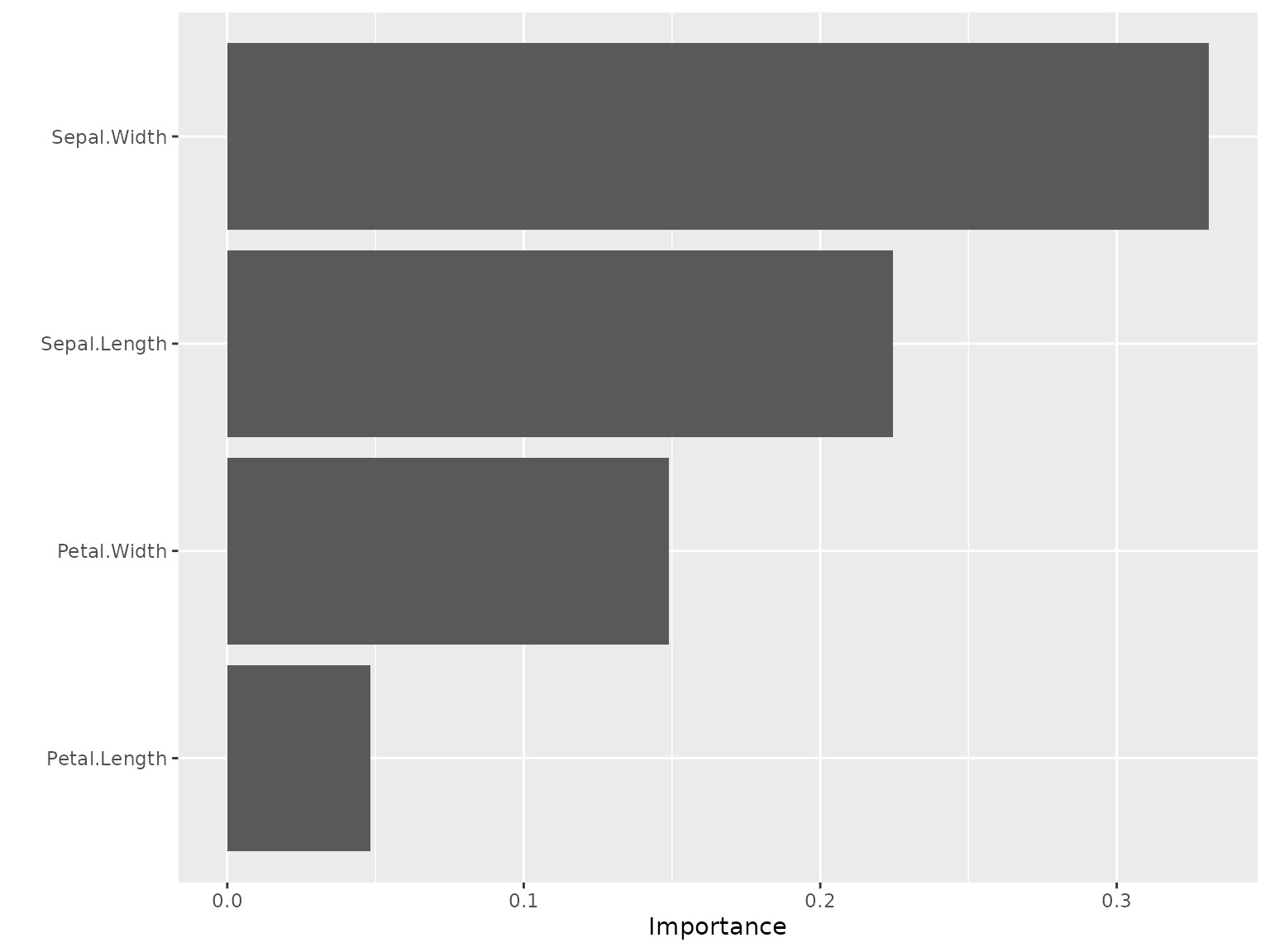
   olden(model, bar_plot = FALSE)
   #>        x_names y_names     rel_imp
   #> 1  Sepal.Width       y  0.33105646
   #> 2 Sepal.Length       y  0.22451097
   #> 3  Petal.Width       y -0.14892091
   #> 4 Petal.Length       y -0.04839239

Integration with {vip}

For users working within the tidymodels ecosystem, kindling models work seamlessly with the vip package:

box::use(
    vip[vi, vip]
)

vi(model) |> 
    vip()

Note: Weight caching increases memory usage proportional to network size. Only enable it when you plan to compute variable importance multiple times on the same model.

Learn More

• Visit the package website: https://kindling.joshuamarie.com
• Report issues: https://github.com/joshuamarie/kindling/issues